OFDM相关学习

循环前缀相关

循环前缀(Cyclic Prefix,CP)的作用:避免符号间干扰和消除子载波间干扰,如何深入理解这个问题,主要从公式的角度进行推导和分析,再结合MATLAB仿真进行验证。

多径信道传输模型

考虑线性时不变系统:
$$
y(t)=h(t)*x(t)=\int h(t)x(t-\tau)d\tau\tag1
$$
其中,$x(t)$表示输入信号,$h(t)$表示信号冲激响应,$y(t)$表示接收信号。离散信号表达式为:
$$
y(n)=\sum_{l=0}^{L-1} h(l)x(n-l)\tag2
$$
上式为多径信道下的信号传输模型,其中$L$表示多径信道的阶数。

OFDM循环前缀的作用

对于OFDM信号而言,发射信号$x(n)$由 IFFT 运算和添加CP得到,其有效信号的表达式为(即IDFT的公式):
$$
x(n)=\frac{1}{\sqrt{N}}\sum_{k=0}^{N-1} X(k)e^{j2\pi \frac{nk}{N}},n=1,\dots,N,k=1,\dots,N
$$
式中,$X(k)$为第$k$个子载波上的发射信号,$N$为IFFT的点数(也是一个OFDM符号时域有效信号 $x(n)$的样点数目。

接下来,需要把式$(2)$中的卷积写成矩阵乘法的形式:

分析过程:假设$L$是多径的的数目,不失一般地,先考虑$y(0)$的表达式,然后利用数学归纳法,写出接收信号的矩阵表达。
$$
y(0)=\sum_{l=0}^{L-1}h(l)x(-l)=h(0)x(0)+h(1)x(-1)+\dots+h(L-1)x(-L+1)
$$

对于单个OFDM符号,CP长度为$N_{CP}$,则接收信号的矩阵表达式为:
$$
\begin{bmatrix}y(-N_{CP})\ \vdots\y(-1)\y(0)\y(1)\y(2)\ \vdots\y(N-2)\y(N-1)\end{bmatrix}=\begin{bmatrix}h(0)&0&0&0&0&0&0&0&0\ \vdots & \ddots&0&0&0&0&0&0&0\h(L-1)&\cdots&h(0)&0&0&0&0&0&0\0&h(L-1)&\cdots&h(0)&0&0&0&0&0\0&0&\ddots&\vdots&h(0)&0&0&0&0\0&0&0&h(L-1)&&h(0)&0&0&0\0&0&0&0&\ddots&&\ddots&0&0\0&0&0&0&0&\ddots&&h(0)&0\0&0&0&0&0&0&h(L-1)&\cdots&h(0)\end{bmatrix}\begin{bmatrix}x(-N_{CP})\\vdots\x(-1)\x(0)\x(1)\x(2)\\vdots\x(N-2)\x(N-1)\end{bmatrix}\tag4
$$
==CP的第一个作用:避免符号间干扰。==由于多径的作用,前一时刻的信号会对当前时刻的信号造成影响。因此,为了保证上一个OFDM不会对当前OFDM符号造成影响,CP的长度必须满足$N_{CP}\ge L$,上式$(4)$中,$N_{CP}= L$。(从两个方向考虑问题,物理意义直观理解,如果多径时延大于$N_{CP}$,接收信号将不全是一个OFDM符号的信息,会有下一个符号信息的干扰,导致后续处理分不开来;数学公式角度理解:上述矩阵成立的边界,即为$N_{CP}\ge L-1$,因为$x,y$这两个列向量长度有系统决定,是确定的形式,L的范围只能存在边界条件,即可得出结论)。

==CP 的第二个作用:消除子载波干扰==。下面进行推导。

循环前缀进一步理解(消除子载波干扰)

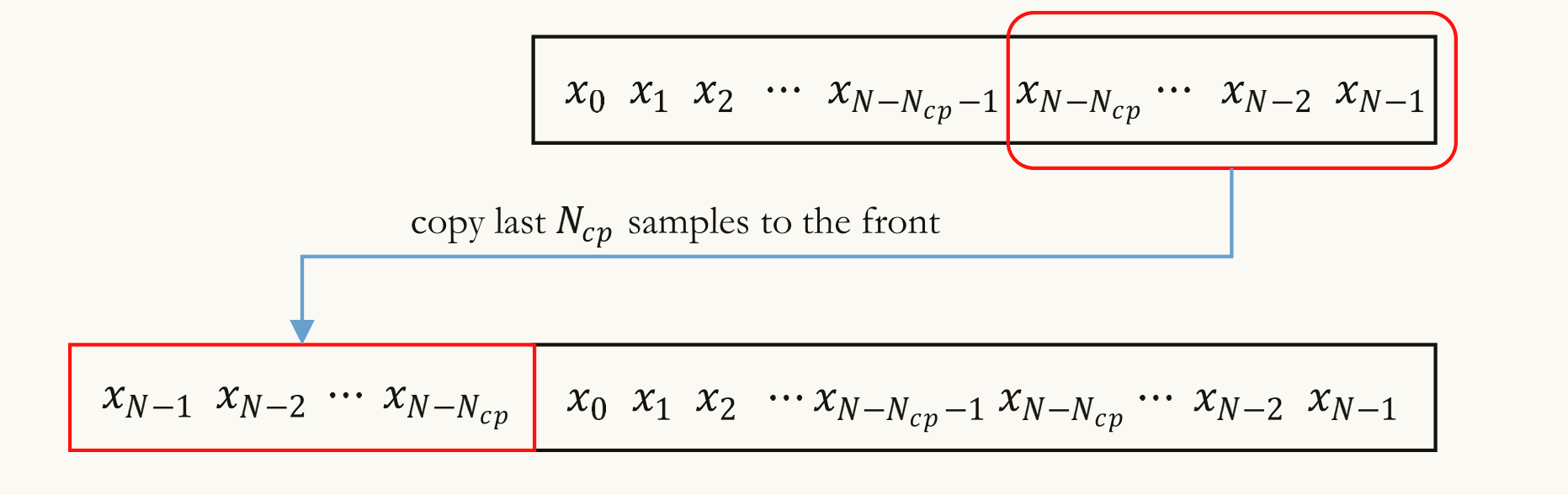
由CP的定义可知,$x(-1)=x(N-1),\dots,x(-N_{CP})=x(N-N_{CP})$。

image-20241028171132568

接收端去掉CP,可以将上式$(4)$进行化简(即考虑$N_{CP}= L$的情况):
$$
\begin{bmatrix}y(0)\y(1)\y(2)\\vdots\y(N-2)\y(N-1)\end{bmatrix}=\begin{bmatrix}0&h(L-1)&\cdots&h(0)&0&0&0&0&0\0&0&\ddots&\vdots&h(0)&0&0&0&0\0&0&0&h(L-1)&&h(0)&0&0&0\0&0&0&0&\ddots&&\ddots&0&0\0&0&0&0&0&\ddots&&h(0)&0\0&0&0&0&0&0&h(L-1)&\cdots&h(0)\end{bmatrix}\begin{bmatrix}x(-N_{CP})\\vdots\x(-1)\x(0)\x(1)\x(2)\\vdots\x(N-2)\x(N-1)\end{bmatrix}\tag5
$$
利用CP的性质,可以进一步得到:
$$
\begin{bmatrix}y(0)\y(1)\y(2)\\vdots\y(N-2)\y(N-1)\end{bmatrix}=\begin{bmatrix}h(0)&0&0&0&h(L-1)&h(1)\\vdots&h(0)&0&0&0&h(L-1)\h(L-1)&&h(0)&0&0&0\0&\ddots&&\ddots&0&0\0&0&\ddots&&h(0)&0\0&0&0&h(L-1)&\cdots&h(0)\end{bmatrix}\begin{bmatrix}x(0)\x(1)\x(2)\\vdots\x(N-2)\x(N-1)\end{bmatrix}\tag6
$$
观察式$(5)$和$(6)$的$h$矩阵,其实质上将式$(5)$中信道矩阵的左上角元素,搬移到式$(6)$中信道矩阵的右上角,这两个等式完全等价,即CP-OFDM将线性**==卷积运算转换为了循环卷积运算==**。

实际上,时域线性卷积≠频域相乘,而是时域循环卷积=频域相乘,引入循环前缀,正好将线性卷积转到循环卷积。

$$
\mathbf{y}=\mathbf{Gx}\tag7
$$

其中,$\mathbf{G}\in \mathbb{C} ^{N\times N}$为时域信道矩阵。根据OFDM接收端的操作,需对接收信号进行FFT运算,可以得到频域信号形式,即
$$
\mathbf{r}=\mathbf{F}\mathbf{y}=\frac{1}{N}\mathbf{F}\mathbf{G}\mathbf{F}^{H}\mathbf{s}\tag8
$$
式中,$\mathbf{F}\in \mathbb{C} ^{N\times N}$表示傅里叶矩阵,性质:$\mathbf{F}\mathbf{F}^{H}=NI$,$\mathbf{s}=[X(1),\dots,X(N)]^T\in ^{N\times 1}$表示频域发射信号。

注意:式中$\mathbf{G}$是一个Toeplitz矩阵,具有循环移位特性。

定义 $\mathbf{H}=\frac{1}{N}\mathbf{F}\mathbf{G}\mathbf{F}^{H}$,利用 托普利兹矩阵_百度百科的性质,则 $\mathbf{H}$是一个对角阵,式 $(8)$可以表示为:
$$
\begin{bmatrix}r(0)\r(1)\r(2)\\vdots\r(N-1)\end{bmatrix}=\begin{bmatrix}H(0)\&\ddots\&&H(k)\&&&\ddots\&&&&H(N-1)\end{bmatrix}\begin{bmatrix}X(0)\\vdots\X(k)\\vdots\X(N-1)\end{bmatrix}\tag9
$$
式中,$H(k)$表示 $\mathbf{H}$的第$k$个对角线元素,从式 $(9)$可以看到,每一个子载波的接收信号与发射信号一一对应,且其他子载波的信号对当前子载波完全没有影响。也就是说,子载波之间不会产生任何干扰,即消除了子载波间干扰。OFDM结合循环前缀,可以使信道均衡、信号解调等在频域并行处理,大大降低了系统复杂度。

有两种说法:CP --> 实现OFDM的循环扩展(为了某种连续性)。

进一步地,分析OFDM频域与时域信道系数的关系,即$H$和$h$的关系:

解决这一问题,需要考虑矩阵的特征值和特征向量:

由$\mathbf{H}$是对角阵可知,$H(k)$是Toeplitz矩阵$\mathbf{G}$的特征值,相应的特征向量为 $\mathbf{F}^{H}$的第 $k$列。理由:$\mathbf{F}^H\mathbf{H}=\mathbf{G}\mathbf{F}^H$.(矩阵分析源头)

考虑矩阵两边的第$k$个列向量,可得$\mathbf{Gf}_k = H(k)\mathbf{f}_k$,其中$\mathbf{f}_k$是$\mathbf{F}^H$的第$k$列,也就是$\mathbf{F}$的第$k$行。这与特征值和特征向量的表达式相同。基于以上讨论,我们下面来说明如何计算$H(k)$。

定义:$W_N = e^{-\frac{j2\pi}{N}}$,$\mathbf{Gf}k = H(k)\mathbf{f}k$的等价形式,即
$$
\frac{1}{\sqrt{N}}\begin{bmatrix}p_0 & p_1 & p_2 & \cdots & p
{N-1} \p
{N-1} & p_0 & p_1 & \cdots & p_{N-2} \p_{N-2} & p_{N-1} & p_0 & \cdots & p_{N-3} \\vdots & \vdots & \vdots & \ddots & \vdots \p_1 & p_2 & p_3 & \cdots & p_0\end{bmatrix}\begin{bmatrix}W_N^{0} \W_N^{-k} \W_N^{-2k} \\vdots \W_N^{-(N-1)k}\end{bmatrix}=\frac{1}{\sqrt{N}}H(k)\begin{bmatrix}W_N^{0} \W_N^{-k} \W_N^{-2k} \\vdots \W_N^{-(N-1)k}\end{bmatrix}\tag{10}
$$
为了计算$H(k)$的表达式,我们观察式(6)和(10)中的Toeplitz矩阵$\mathbf{G}$和$\mathbf{P}$,有$\mathbf{P}{m,n} = p{(n-m)\mod N}$, $p_l = h_{(N-l)\mod N}$,其中$m, n, l = 0, 1, 2, \ldots, N-1$。

因此,式(10)等号左边:矩阵$\mathbf{P}$的第$(m+1)$行与IDFT矩阵第$k$列的内积有
$$
\frac{1}{\sqrt{N}} \sum_{n=0}^{N-1} p_{(n-m)N} W_N^{-nk} = \frac{1}{\sqrt{N}} W_N^{-mk} \sum{n=0}^{N-1} p_{(n-m)N} W_N^{-(n-m)N k} = \frac{1}{\sqrt{N}} W_N^{-mk} \sum{l=0}^{N-1} p_l W_N^{-lk}\tag{11}
$$
式中,第1个等号利用了性质$W_N^{-(n-m)k} = W_N^{-(n-m)N k}$(以$N$为周期的周期性)。为进一步计算式(11)的求和项,我们定义$H_k = \sum{l=0}^{N-1} p_l W_N^{-lk}$ ,即
$$
H_k = \sum
{l=0}^{N-1} p_l W_N^{-lk} = \sum_{l=0}^{N-1} h_{(N-l)N} W_N^{-lk} = \sum{l=0}^{N-1} h_{(N-l)N} W_N^{(N-l)N k} = \sum{l’=0}^{N-1} h{l’} W_N^{l’k}\tag{12}
$$
式中,第3个等号利用了性质$W_N^{Nk} = 1$,$W_N^{(N-l)k} = W_N^{(N-l)_N k}$。

可以看到,频域信道系数$H_k$恰巧是时域信道系数$h_{l’}, l’ = 0, 1, \ldots, N-1$的傅里叶变换!

线性卷积和循环卷积的转换

参考书籍《Wireless Communication Systems in Matlab, Second Edition

下面给出一个简单的MATLAB程序:

1
2
3
4
5
6
7
8
9
10
11
12
13
14
15
16
17
18
19
20
21
22
23
clc; clear; close all;
%========================================================================%
%:此程序用来测试《Wireless Communication Systems in Matlab, Second Edition》
%:第14章OFDM的前向解调算法
%========================================================================%
%% 线性卷积与循环卷积转化
N = 8; %period of DFT
s = randn(1, 8)
h = randn(1, 3)
lin_s_h = conv(h, s) %linear convolution of h and s
cir_s_h = cconv(h, s, N) %#ok<*NOPTS> %circular convolution of h and s with period N
Ncp = 2; %number of symbols to copy and paste for CP
s_cp = [s(end - Ncp + 1:end) s]; %copy last Ncp syms from s, add as prefix
lin_scp_h = conv(h, s_cp) %linear conv. of CP-OFDM symbol s_cp and CIR h
r = lin_scp_h(Ncp + 1:N + Ncp) %cut from index Ncp+1 to N+Ncp
%% 验证循环卷积=IDFT{DFT{h[n]} x DFT{s[n]}}
R = fft(r, N); %frequency response of received signal
H = fft(h, N); %frequency response of CIR
S = fft(s, N); %frequency response of OFDM signal (non CP)
r1 = ifft(S .* H); %IFFT of product of individual DFTs
display(['IFFT(DFT(H)*DFT(S)) : ', num2str(r1)])
display(['cconv(s,h): ', num2str(r)])

OFDM信号仿真部分代码

以下为一个OFDM误码率仿真示例:

1
2
3
4
5
6
7
8
9
10
11
12
13
14
15
16
17
18
19
20
21
22
23
24
25
26
27
28
29
30
31
32
33
34
35
36
37
38
39
40
41
42
43
44
45
46
47
48
49
50
51
52
53
54
55
56
57
58
59
60
61
62
63
64
65
66
67
68
69
70
71
72
73
74
75
76
77
78
79
80
81
82
83
84
85
86
87
88
89
90
91
92
93
94
95
96
97
98
99
100
101
102
103
104
105
106
107
108
109
110
111
112
113
114
115
116
117
118
119
120
121
122
123
124
125
126
127
128
129
130
131
132
133
134
135
136
137
138
139
140
141
142
143
144
145
clc; clear; close all
% DATA: 2024-9-12-22:00
% Author: Poster
% Description: This is a simulation of OFDM over AWGN channel.
%:注:Tx-Signal采用列向量的形式;
%:注:MATLAB采用优先采用列向量进行存储,按列运算速度相对较快
%------------Simulation parameters---------%
MOD_TYPE = 'PSK'; % Modulation type'
M = 4; % Constellation size
phase_init = pi / M; % Initial phase
N = 64; % FFT size
Ncp = 16; % number of symbols in the cyclic prefix
Num = 1e5; % Number of OFDM Symbols to transmit
EbN0dB = 0:2:20; % bit to noise ratio
k = log2(M); % number of bits per symbol
EsN0dB = 10 * log10(k) + EbN0dB; % convert to symbol energy to noise ratio
errors = zeros(1, length(EsN0dB)); %to store symbol errors

for i = 1:length(EsN0dB)
for Sym = 1:Num % Monte Carlo Simulation
%--------Constellation Mapping-------%
symbols_data = randi([0 M - 1], N, 1); % Random symbols
X = pskmod(symbols_data, M, phase_init); % PSK modulation
%--------------Transmitter-----------%
x = ifft(X, N); % IDFT
s = add_cyclic_prefix(x, Ncp); % Add CP
%----------------Channel-------------%
r = add_awgn_noise(s, EsN0dB(i)); % Add AWGN noise r = s + n
%---------------Receiver-------------%
y = remove_cyclic_prefix(r, Ncp, N); % remove CP
Y = fft(y, N); % DFT
symbols_data_cap = pskdemod(Y, M, phase_init); % PSK demodulation
%------------error count-------------%
numErrors = sum(symbols_data ~= symbols_data_cap); % Count errors
errors(i) = errors(i) + numErrors; % Update error count
end
end
simulatedSER = errors / (Num * N); % Symbol Error Rate
theoreticalSER = ser_awgn(EbN0dB, MOD_TYPE, M);
% Plot theoretical curves and simulated BER points
plot(EbN0dB, log10(simulatedSER), 'ro'); hold on;
plot(EbN0dB, log10(theoreticalSER), 'r-'); grid on;
title(['Performance of ', num2str(M), '-', MOD_TYPE, ' OFDM over AWGN channel']);
xlabel('Eb/N0 (dB)'); ylabel('Symbol Error Rate');
legend('simulated', 'theoretical');
%=============Function Definition==========%
function s = add_cyclic_prefix(x, Ncp)
%function to add cyclic prefix to the generated OFDM symbol x that
%is generated at the output of the IDFT block
% x - ofdm symbol without CP (output of IDFT block)
% Ncp-num. of samples at x's end that will copied to its beginning
% s - returns the cyclic prefixed OFDM symbol
s = [x(end - Ncp + 1:end); x]; %Cyclic prefixed OFDM symbol
end
function [r, n, N0] = add_awgn_noise(s, SNRdB, L)
%Function to add AWGN to the given signal
%[r,n,N0]= add_awgn_noise(s,SNRdB) adds AWGN noise vector to signal
%'s' to generate a %resulting signal vector 'r' of specified SNR
%in dB. It also returns the noise vector 'n' that is added to the
%signal 's' and the spectral density N0 of noise added
%
%[r,n,N0]= add_awgn_noise(s,SNRdB,L) adds AWGN noise vector to
%signal 's' to generate a resulting signal vector 'r' of specified
%SNR in dB. The parameter 'L' specifies the oversampling ratio used
%in the system (for waveform simulation). It also returns the noise
%vector 'n' that is added to the signal 's' and the spectral
%density N0 of noise added
s_temp = s;
if iscolumn(s), s = s.'; end %to return the result in same dim as 's'
gamma = 10 ^ (SNRdB / 10); %SNR to linear scale
if nargin == 2, L = 1; end %if third argument is not given, set it to 1
if isvector(s)
P = L * sum(abs(s) .^ 2) / length(s); %Actual power in the vector
else %for multi-dimensional signals like MFSK
P = L * sum(sum(abs(s) .^ 2)) / length(s); %if s is a matrix [MxN]
end
N0 = P / gamma; %Find the noise spectral density

if (isreal(s))
n = sqrt(N0 / 2) * randn(size(s)); %computed noise
else
n = sqrt(N0 / 2) * (randn(size(s)) + 1i * randn(size(s))); %computed noise
end
r = s + n; %received signal
if iscolumn(s_temp), r = r.'; end %return r in original format as s
end
function y = remove_cyclic_prefix(r, Ncp, N)
%function to remove cyclic prefix from the received OFDM symbol r
% r - received ofdm symbol with CP
% Ncp - num. of samples at beginning of r that need to be removed
% N - number of samples in a single OFDM symbol
% y - returns the OFDM symbol without cyclic prefix
y = r(Ncp + 1:N + Ncp); %cut from index Ncp+1 to N+Ncp
end
function [SER] = ser_awgn(EbN0dB, MOD_TYPE, M, COHERENCE)
%Theoretical Symbol Error Rate for various modulations over AWGN
%EbN0dB - list of SNR per bit values
%MOD_TYPE - 'BPSK','PSK','QAM','PAM','FSK'
%M - Modulation level for the chosen modulation
% - For PSK,PAM,FSK M can be any power of 2
% - For QAM M must be even power of 2 (square QAM only)
%Parameter COHERENCE is only applicable for FSK modulation
%COHERENCE = 'coherent' for coherent FSK detection
% = 'noncoherent' for noncoherent FSK detection
gamma_b = 10 .^ (EbN0dB / 10); %SNR per bit in linear scale
gamma_s = log2(M) * gamma_b; %SNR per symbol in linear scale
SER = zeros(size(EbN0dB));
switch lower(MOD_TYPE)
case 'bpsk'
SER = 0.5 * erfc(sqrt(gamma_b));
case {'psk', 'mpsk'}
if M == 2 %for BPSK
SER = 0.5 * erfc(sqrt(gamma_b));
else
if M == 4 %for QPSK
Q = 0.5 * erfc(sqrt(gamma_b)); SER = 2 * Q - Q .^ 2;
else %for other higher order M-ary PSK
SER = erfc(sqrt(gamma_s) * sin(pi / M));
end
end
case {'qam', 'mqam'}
SER = 1 - (1 - (1 - 1 / sqrt(M)) * erfc(sqrt(3/2 * gamma_s / (M - 1)))) .^ 2;
case {'fsk', 'mfsk'}
if strcmpi(COHERENCE, 'coherent')
for ii = 1:length(gamma_s)
fun = @(q) (0.5 * erfc((-q - sqrt(2 .* gamma_s(ii))) / sqrt(2))) .^ (M - 1) .* 1 / sqrt(2 * pi) .* exp(-q .^ 2/2);
SER(ii) = 1 - integral(fun, -inf, inf);
end
else %Default compute for noncoherent
for jj = 1:length(gamma_s)
summ = 0;
for i = 1:M - 1
n = M - 1; r = i; %for nCr formula
summ = summ + (-1) .^ (i + 1) ./ (i + 1) .* prod((n - r + 1:n) ./ (1:r)) .* exp(-i ./ (i + 1) .* gamma_s(jj));
end
SER(jj) = summ; %Theoretical SER for non-coherent detection
end
end
case {'pam', 'mpam'}
SER = 2 * (1 - 1 / M) * 0.5 * erfc(sqrt(3 * gamma_s / (M ^ 2 - 1)));
otherwise
disp('ser_awgn.m: Invalid modulation (MOD_TYPE) selected');
end
end